Stitching Images (large dataset)
[1]:
import h5py
import matplotlib.pyplot as plt
import numpy as np

import microscopy_data_analysis as mda
[2]:
#for the next line to work, the file create_example_for_grid_stitching.py
#should be in the same directory as this notebook
import create_data_for_grid_stitching

create_data_for_grid_stitching.run_script()
[3]:
example_path="example_images"
pathlist=mda.get_files_of_format(example_path,"tif")
N=len(pathlist)
pathlist[:3]
[3]:
['example_images/image_00.tif',
 'example_images/image_01.tif',
 'example_images/image_02.tif']
[4]:
%matplotlib inline
positions=np.zeros([N,2])
counter=0
for i in range(5):
    for j in range(5):
        if counter==len(positions):
            break
        positions[counter]=j*385,5*375-i*375
        counter+=1

plt.figure(figsize=[10,10])
plt.plot(positions[:,0],positions[:,1],'o')
for i in range(len(positions)):
    plt.text(positions[i,0],positions[i,1],str(i))
plt.xlabel(r"x [mm]")
plt.ylabel(r"y [mm]")
plt.axis("equal")
plt.show()
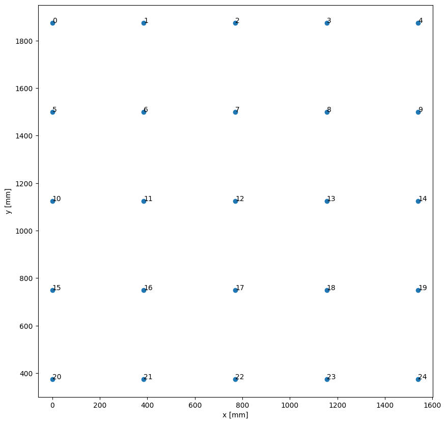
Even though set of images is small, this example shows a workflow, as if the size of the image stack would be large (potentially bigger than RAM).
Side note: In this example we use a grid of images again, but any other arangement of overlapping images would work as well.
[5]:
stack=mda.image_stack(mode='storage')
For .h5 provide the path to the h5-file (that serves as h5-directory) via the 'set_directory_path' method
For .tif, .png, ... image files  either provide  a list of relative or absolute filepaths via 'set_img_list'
or provide the folder containing only the contributing images via 'set_directory_path'
[6]:
# identical to minimal example
stack.set_img_list(pathlist)
stack.sniff_dimensions()
stack.set_units_per_pixel(1.1)
stack.set_positions(positions)
polygons,anchor_points=stack.make_polygons()
[7]:
stack.create_h5cube_duplicate_for_modifying("example_data.h5",dset_name="data")
100%|██████████| 25/25 [00:00<00:00, 213.42it/s]
[8]:
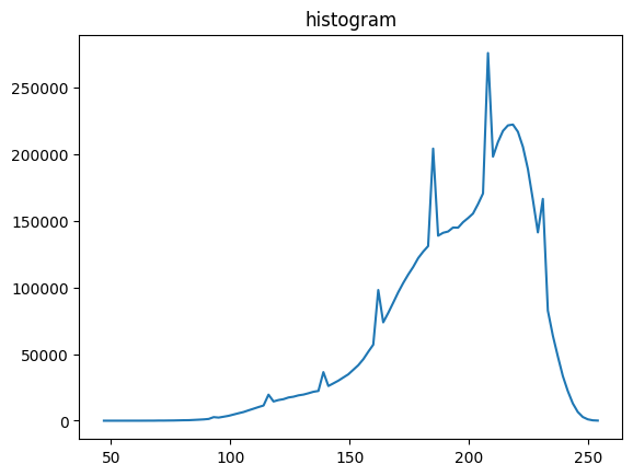
# let's have a look into the histogram of brightness values
# of all images in the stack

vmin,vmax,vbins,vhist=stack.stats(dset_name="data")
plt.title("histogram")
plt.plot(mda.bin_centering(vbins), vhist)
plt.show()
min/max: 100%|██████████| 25/25 [00:00<00:00, 822.41it/s]
histo: 100%|██████████| 25/25 [00:00<00:00, 772.72it/s]
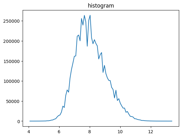
[9]:
# z-transform (subtraction of mean and division by standard deviation) is
# usually a good idea, since the contrast of images is often rescaled
# to the file format, when saved
stack.z_transform_images()
# no dset_name given, will overwrite existing dataset
# (only in the modifiable h5 file)

vmin,vmax,vbins,vhist=stack.stats(dset_name="data")
plt.title("histogram")
plt.plot(mda.bin_centering(vbins), vhist)
plt.show()
z-transform: 100%|██████████| 25/25 [00:00<00:00, 142.97it/s]
positive offset: 100%|██████████| 25/25 [00:00<00:00, 450.89it/s]
min/max: 100%|██████████| 25/25 [00:00<00:00, 895.26it/s]
histo: 100%|██████████| 25/25 [00:00<00:00, 563.05it/s]
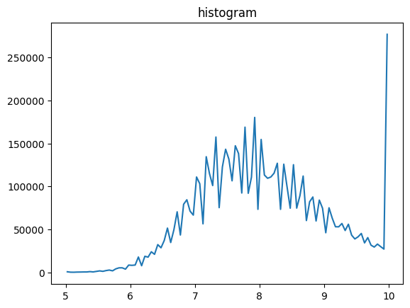
[10]:
stack.clip(5,10,new_dset_name="clipped")
# now for example this clipping might not be very useful,
# so we do not overwrite 'data' but create 'clipped' instead

vmin,vmax,vbins,vhist=stack.stats(dset_name="clipped")
plt.title("histogram")
plt.plot(mda.bin_centering(vbins), vhist)
plt.show()
100%|██████████| 25/25 [00:00<00:00, 453.85it/s]
min/max: 100%|██████████| 25/25 [00:00<00:00, 1238.30it/s]
histo: 100%|██████████| 25/25 [00:00<00:00, 617.39it/s]
[11]:
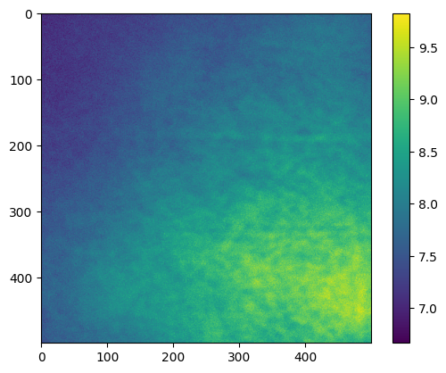
# Instead of clipping, let's assume all images were taken with the same camera.
# Then, all images might show the same inhomogeneities in illumination for example.
# Therefore, we want to extract an image representing just these inhomogeneities
# and normalize (divide) the data with it.
flat_field=stack.flat_field_generation(subdiv=2)
# The number of subdivisions determine how much of the data is loaded into RAM
# simultaneously (subdiv=2 corresponds to half of it).
plt.imshow(flat_field)
plt.colorbar()
plt.show()
1 out of 2 iterations
2 out of 2 iterations
[12]:
# Typically, we expect a smooth flat field image, that does not show any objects
# displayed in the images. The more images we can provide for the flat field generation,
# the better. Here, we see already with just 25 images, it is not very smooth, but ok.
stack.flat_field_correction(flat_field=flat_field,dset_name="data",new_dset_name="corrected_data")
100%|██████████| 25/25 [00:00<00:00, 262.53it/s]
[13]:
%matplotlib inline
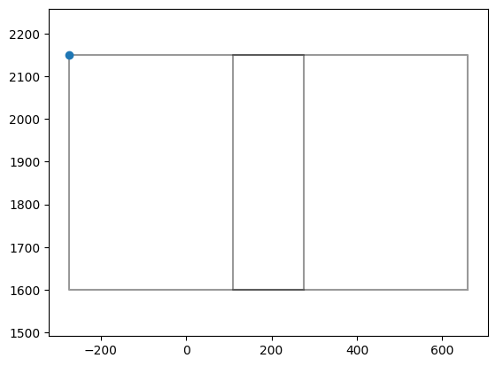
# Now back to the stitching:
# check for two images, if there is overlap
# also origin (anchor) of the pixel coordinates, shown as blue dot, should be
# in the left upper corner of an image
index=0
plt.plot(np.array(polygons[index].exterior.xy[0]),np.array(polygons[index].exterior.xy[1]),'k-',alpha=0.4)
plt.plot(anchor_points[index][0],anchor_points[index][1],'o')
index=1
plt.plot(np.array(polygons[index].exterior.xy[0]),np.array(polygons[index].exterior.xy[1]),'k-',alpha=0.4)
plt.axis("equal")
plt.show()
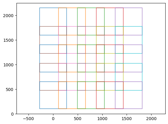
[14]:
# show all images (abstracted as polygons)
for index in range(len(stack.polygons)):
    plt.plot(np.array(stack.polygons[index].exterior.xy[0]),np.array(stack.polygons[index].exterior.xy[1]),'-',alpha=0.6)
plt.axis("equal")
plt.show()
[15]:
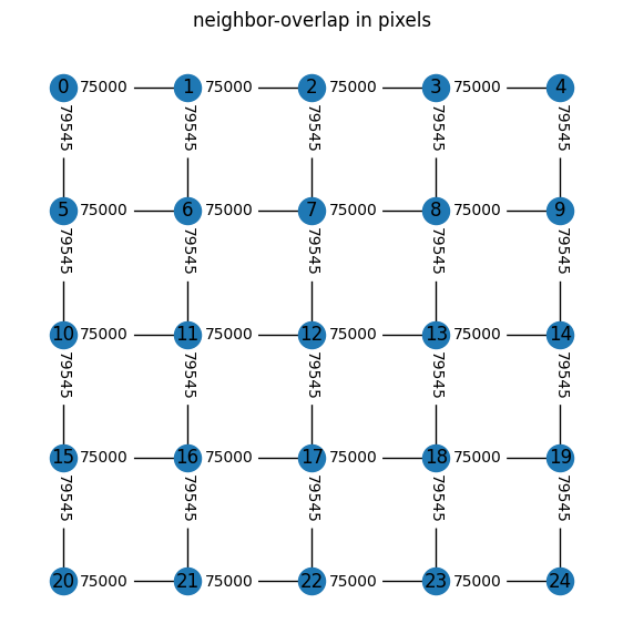
connected_groups=stack.connection_groups()
stack.plot_connection_network(figsize=[10,10],relative=False)
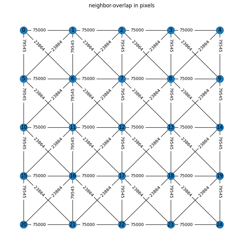
[16]:
# to accelerate calculation one can neglect diagonal connections
connected_groups=stack.connection_groups(minimal_number_of_pixels=50_000)
stack.plot_connection_network(figsize=[7,7],relative=False)
[17]:
pair_shifts=stack.check_pairs(dset_name='corrected_data')
100%|██████████| 40/40 [00:02<00:00, 18.38it/s]
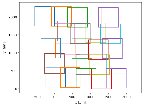
[18]:
moved_polygons=stack.optimize_positions()
   Iteration     Total nfev        Cost      Cost reduction    Step norm     Optimality
       0              1         1.2884e+05                                    1.70e+02
       1              3         6.9981e+04      5.89e+04       2.16e+02       9.76e+01
       2              4         6.0966e+04      9.01e+03       4.31e+02       2.01e+02
       3              5         2.3257e+04      3.77e+04       1.08e+02       8.98e+01
       4              7         1.7069e+04      6.19e+03       5.39e+01       4.11e+01
       5              8         1.5646e+04      1.42e+03       5.39e+01       4.46e+01
       6             10         1.4697e+04      9.50e+02       1.35e+01       1.58e+01
       7             11         1.4228e+04      4.69e+02       2.70e+01       2.55e+01
       8             12         1.4203e+04      2.44e+01       2.70e+01       3.28e+01
       9             13         1.3837e+04      3.67e+02       6.74e+00       1.66e+01
      10             14         1.3651e+04      1.86e+02       1.35e+01       1.42e+01
      11             15         1.3599e+04      5.19e+01       1.35e+01       1.59e+01
      12             16         1.3503e+04      9.57e+01       3.37e+00       8.16e+00
      13             17         1.3441e+04      6.15e+01       6.74e+00       6.50e+00
      14             18         1.3404e+04      3.76e+01       6.74e+00       7.30e+00
      15             19         1.3380e+04      2.34e+01       6.74e+00       7.66e+00
      16             20         1.3356e+04      2.48e+01       1.69e+00       3.96e+00
      17             21         1.3336e+04      1.97e+01       3.37e+00       2.90e+00
      18             22         1.3321e+04      1.49e+01       3.37e+00       3.18e+00
      19             23         1.3311e+04      1.01e+01       3.37e+00       3.53e+00
      20             24         1.3304e+04      6.94e+00       3.37e+00       4.09e+00
      21             25         1.3298e+04      6.30e+00       8.43e-01       2.07e+00
      22             26         1.3292e+04      5.48e+00       1.69e+00       1.38e+00
      23             27         1.3288e+04      4.47e+00       1.69e+00       1.48e+00
      24             28         1.3285e+04      3.14e+00       1.69e+00       1.59e+00
      25             29         1.3282e+04      2.15e+00       1.69e+00       1.95e+00
      26             30         1.3281e+04      1.76e+00       1.69e+00       1.76e+00
      27             31         1.3279e+04      1.54e+00       4.21e-01       8.80e-01
      28             32         1.3278e+04      1.26e+00       8.43e-01       8.00e-01
      29             33         1.3277e+04      9.93e-01       8.43e-01       7.17e-01
      30             34         1.3276e+04      7.06e-01       8.43e-01       9.09e-01
      31             35         1.3276e+04      5.30e-01       8.43e-01       7.96e-01
      32             36         1.3275e+04      3.68e-01       8.43e-01       9.77e-01
      33             37         1.3275e+04      3.95e-01       2.11e-01       5.84e-01
      34             38         1.3275e+04      3.09e-01       4.21e-01       3.53e-01
      35             39         1.3274e+04      2.40e-01       4.21e-01       4.50e-01
      36             40         1.3274e+04      1.68e-01       4.21e-01       3.65e-01
      37             41         1.3274e+04      1.20e-01       4.21e-01       5.15e-01
      38             42         1.3274e+04      1.01e-01       4.21e-01       3.62e-01
      39             43         1.3274e+04      9.55e-02       1.05e-01       2.32e-01
      40             44         1.3274e+04      7.20e-02       2.11e-01       2.27e-01
      41             45         1.3274e+04      5.57e-02       2.11e-01       1.87e-01
      42             46         1.3274e+04      3.90e-02       2.11e-01       2.57e-01
      43             47         1.3274e+04      3.10e-02       2.11e-01       1.85e-01
      44             48         1.3274e+04      2.05e-02       2.11e-01       2.71e-01
      45             49         1.3274e+04      2.48e-02       5.27e-02       1.59e-01
      46             50         1.3274e+04      1.83e-02       1.05e-01       9.32e-02
      47             51         1.3274e+04      1.36e-02       1.05e-01       1.25e-01
      48             52         1.3274e+04      9.68e-03       1.05e-01       9.75e-02
      49             53         1.3274e+04      6.89e-03       1.05e-01       1.40e-01
      50             54         1.3274e+04      6.23e-03       2.63e-02       8.22e-02
      51             55         1.3274e+04      5.44e-03       5.27e-02       4.88e-02
      52             56         1.3274e+04      4.53e-03       5.27e-02       5.89e-02
      53             57         1.3274e+04      3.25e-03       5.27e-02       4.98e-02
      54             58         1.3274e+04      2.26e-03       5.27e-02       7.17e-02
      55             59         1.3274e+04      1.84e-03       5.27e-02       4.97e-02
      56             60         1.3274e+04      1.52e-03       1.32e-02       3.24e-02
      57             61         1.3274e+04      1.31e-03       2.63e-02       3.02e-02
      58             62         1.3274e+04      1.06e-03       2.63e-02       2.51e-02
      59             63         1.3274e+04      7.80e-04       2.63e-02       3.50e-02
      60             64         1.3274e+04      5.71e-04       2.63e-02       2.59e-02
      61             65         1.3274e+04      4.04e-04       2.63e-02       3.85e-02
      62             66         1.3274e+04      3.90e-04       6.58e-03       2.22e-02
      63             67         1.3274e+04      3.27e-04       1.32e-02       1.27e-02
      64             68         1.3274e+04      2.68e-04       1.32e-02       1.62e-02
      65             69         1.3274e+04      1.91e-04       1.32e-02       1.32e-02
      66             70         1.3274e+04      1.34e-04       1.32e-02       1.95e-02
      67             71         1.3274e+04      1.11e-04       1.32e-02       1.34e-02
      68             72         1.3274e+04      9.51e-05       3.29e-03       8.43e-03
`ftol` termination condition is satisfied.
Function evaluations 72, initial cost 1.2884e+05, final cost 1.3274e+04, first-order optimality 8.43e-03.
[19]:
%matplotlib inline
for i in range(len(moved_polygons)):
    plt.plot(np.array(moved_polygons[i].exterior.xy[0]),np.array(moved_polygons[i].exterior.xy[1]))#'k-')
plt.xlabel(r"x [$\mu$m]")
plt.ylabel(r"y [$\mu$m]")
plt.axis("equal")
plt.show()
[20]:
stack.map_from_polygons_h5(moved_polygons,boolean_mask=True,blending="quadratic",dset_name="corrected_data")
  0%|          | 0/25 [00:00<?, ?it/s]100%|██████████| 25/25 [00:00<00:00, 43.96it/s]
Rows: 100%|██████████| 5/5 [00:00<00:00, 92.95it/s]
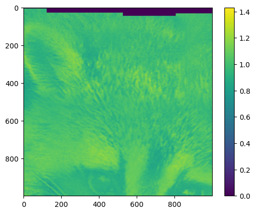
For very large maps, the map typically can not be displayed fully by plt.imshow. Small parts are no problem, like:
[21]:
# inspect the image map
with h5py.File("example_data.h5",'r') as f:
    img=f["map"]
    #this does not load the image into RAM yet, only when sliced
    # --> img=f["map"][:]  would load all data into RAM (and should be avoided)
    imgsection=img[0:1000,800:1800] # loads a 1000x1000 slice into RAM
plt.imshow(imgsection)
plt.colorbar()
plt.show()
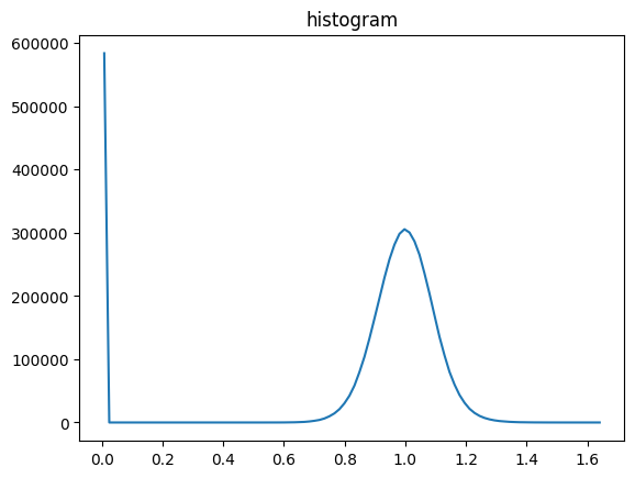
[22]:
# inspect the brightness value histogram
vmin,vmax,vbins,vhist=stack.stats(dset_name="map")
plt.title("histogram")
plt.plot(mda.bin_centering(vbins), vhist)
plt.show()
Rows: 100%|██████████| 5/5 [00:00<00:00, 141.18it/s]
Rows: 100%|██████████| 5/5 [00:00<00:00, 99.15it/s]
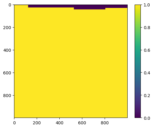
[23]:
# Most of the zeros in the first histogram are from the borders of the image map.
# To ignore these values, we can use the boolean_mask,
# which yields False in such regions.
with h5py.File("example_data.h5",'r') as f:
    img=f["boolean_mask"]
    #this does not load the image into RAM yet, only when sliced
    # --> img=f["map"][:]  would load all data into RAM (and should be avoided)
    imgsection=img[0:1000,800:1800] # loads a 1000x1000 slice into RAM
plt.imshow(imgsection)
plt.colorbar()
plt.show()
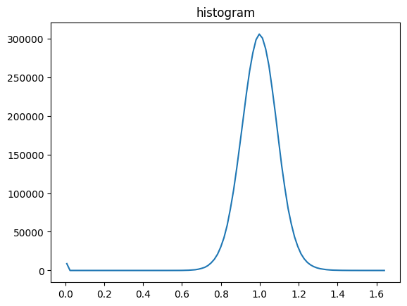
[24]:
# brightness histogram with boolean mask
vmin,vmax,vbins,vhist=stack.stats(dset_name="map",mask="boolean_mask")
plt.title("histogram")
plt.plot(mda.bin_centering(vbins), vhist)
plt.show()
Rows: 100%|██████████| 5/5 [00:00<00:00, 65.86it/s]
Rows: 100%|██████████| 5/5 [00:00<00:00, 68.00it/s]
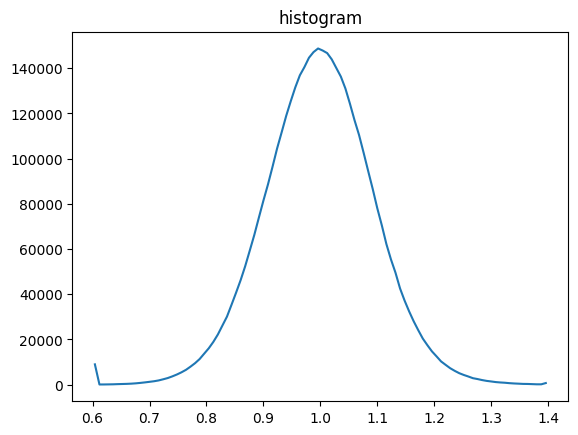
[25]:
# clip the range of brightness values for better contrast
stack.clip(0.6,1.4,dset_name="map",new_dset_name="clipped")

vmin,vmax,vbins,vhist=stack.stats(dset_name="clipped",mask="boolean_mask")
plt.title("histogram")
plt.plot(mda.bin_centering(vbins), vhist)
plt.show()
Rows: 100%|██████████| 5/5 [00:00<00:00, 103.88it/s]
Rows: 100%|██████████| 5/5 [00:00<00:00, 155.72it/s]
Rows: 100%|██████████| 5/5 [00:00<00:00, 100.53it/s]
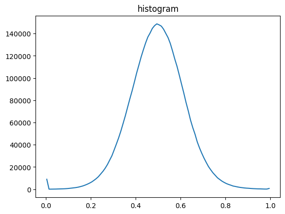
[26]:
# rescale the values between 0 and 1 for saving the image in float32
# (alternatively rescaling to 0 and 255 for uint8, would be an option as well)
# stack.normalize(dset_name="clipped",new_max=255)

stack.normalize(dset_name="clipped")

vmin,vmax,vbins,vhist=stack.stats(dset_name="clipped",mask="boolean_mask")
plt.title("histogram")
plt.plot(mda.bin_centering(vbins), vhist)
plt.show()
Rows: 100%|██████████| 5/5 [00:00<00:00, 192.61it/s]
Rows: 100%|██████████| 5/5 [00:00<00:00, 69.62it/s]
Rows: 100%|██████████| 5/5 [00:00<00:00, 115.91it/s]
Rows: 100%|██████████| 5/5 [00:00<00:00, 98.09it/s]
[27]:
# for viewing the images with standard software, big_tiff=False can be used
# for very big maps big_tiff=True must be used and images can be opened
# for example with imagej/Fiji  (for fast zooming use: mda.h5_to_pyramidal_tiff)
mda.h5_to_tiff(h5_path="example_data.h5",dset_name="clipped",out_path="stitching_example_large.tif",big_tiff=False,dtype='f4')
Saved TIFF: stitching_example_large.tif
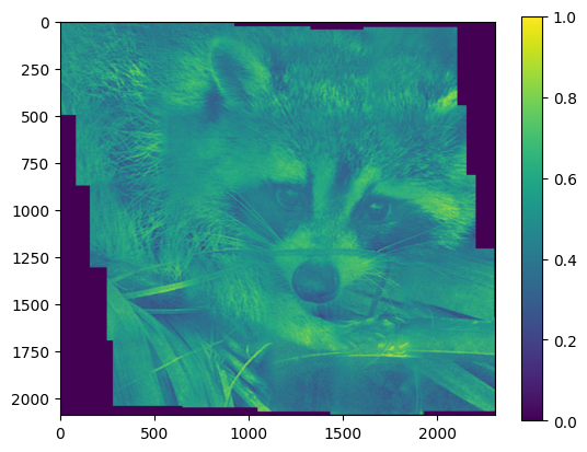
[28]:
# Since, this dataset is not big, we can show the image
# and compare it with the minimal example,
# where the images were stitched without further processing.
# (it is not completely fair, because we also used blending='quadratic')
with h5py.File("example_data.h5",'r') as f:
    img=f["clipped"][:] # dont't do this for a very large map
plt.imshow(img)
plt.colorbar()
plt.show()
[ ]: